Note
Click here to download the full example code
Customize resampling target
This example demonstrates how to customize the resampling target to achieve advanced resampling control. This can be easily done by setting the “target_label” and “n_target_samples” parameter when calling the “fit()” method.
Note that this feature only applies to resampling-based ensemble classifiers that are iteratively trained.
This example uses:
# Authors: Zhining Liu <zhining.liu@outlook.com>
# License: MIT
print(__doc__)

# Import imbalanced-ensemble
import imbens

# Import utilities
from sklearn.datasets import make_classification
from sklearn.model_selection import train_test_split
from imbens.ensemble.base import sort_dict_by_key
from collections import Counter

# Import plot utilities
from imbens.utils._plot import set_ax_border
import matplotlib.pyplot as plt
import seaborn as sns
sns.set_context('talk')

RANDOM_STATE = 42

init_kwargs = {
    'n_estimators': 1,
    'random_state': RANDOM_STATE,
}
fit_kwargs = {
    'train_verbose': {
        'print_metrics': False,
    },
}

# sphinx_gallery_thumbnail_number = -1
Prepare data
Make a toy 3-class imbalanced classification task.
# Generate and split a synthetic dataset
X, y = make_classification(n_classes=3, n_samples=2000, class_sep=2,
    weights=[0.1, 0.3, 0.6], n_informative=3, n_redundant=1, flip_y=0,
    n_features=20, n_clusters_per_class=2, random_state=RANDOM_STATE)
X_train, X_valid, y_train, y_valid = train_test_split(X, y,
    test_size=0.5, stratify=y, random_state=RANDOM_STATE)

# Print class distribution
print('Training dataset distribution    %s' % sort_dict_by_key(Counter(y_train)))
print('Validation dataset distribution  %s' % sort_dict_by_key(Counter(y_valid)))
Training dataset distribution    {0: 100, 1: 300, 2: 600}
Validation dataset distribution  {0: 100, 1: 300, 2: 600}
Implement some plot utilities
ylim = (0, 630)

all_distribution = {}

def plot_class_distribution(distr:dict, xlabel:str='Class Label',
                            ylabel:str='Number of samples', **kwargs):
    distr = dict(sorted(distr.items(), key=lambda k: k[0], reverse=True))
    ax = sns.barplot(
        x=list(distr.keys()),
        y=list(distr.values()),
        order=list(distr.keys()),
        **kwargs
    )
    set_ax_border(ax)
    ax.grid(axis='y', alpha=0.5, ls='-.')
    ax.set_xlabel(xlabel)
    ax.set_ylabel(ylabel)
    return ax

def plot_class_distribution_comparison(clf,
                                       title1='Original imbalanced class distribution',
                                       title2='After resampling', figsize=(12, 6)):
    fig, (ax1, ax2) = plt.subplots(1, 2, figsize=figsize)
    plot_class_distribution(clf.origin_distr_, ax=ax1)
    ax1.set(ylim=ylim, title=title1)
    plot_class_distribution(clf.target_distr_, ax=ax2)
    ax2.set(ylim=ylim, title=title2)
    fig.tight_layout()
Default under-sampling
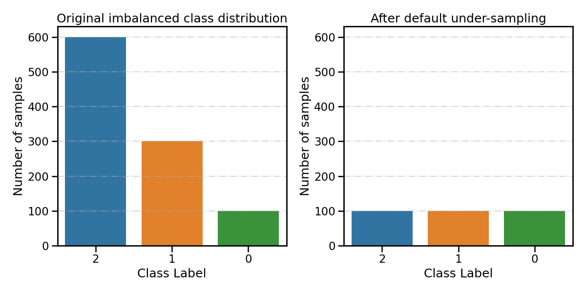
By default, under-sampling-based ensemble methods will consider the smallest class as the minority class (class 0 with 100 samples). All other classes (class 1 and 2) will be considered as majority classes and will be under-sampled until the number of samples is equalized.
Take SelfPacedEnsembleClassifier as example
spe_clf = imbens.ensemble.SelfPacedEnsembleClassifier(**init_kwargs)
Train with the default under-sampling setting
spe_clf.fit(X_train, y_train, **fit_kwargs)

all_distribution['Before under-sampling'] = spe_clf.origin_distr_
resampling_type='After default under-sampling'
all_distribution[resampling_type] = spe_clf.target_distr_
plot_class_distribution_comparison(spe_clf, title2=resampling_type)
┏━━━━━━━━━━━━━┳━━━━━━━━━━━━━━━━━━━━━━━━━━┓
┃             ┃                          ┃
┃ #Estimators ┃    Class Distribution    ┃
┃             ┃                          ┃
┣━━━━━━━━━━━━━╋━━━━━━━━━━━━━━━━━━━━━━━━━━┫
┃      1      ┃ {0: 100, 1: 100, 2: 100} ┃
┣━━━━━━━━━━━━━╋━━━━━━━━━━━━━━━━━━━━━━━━━━┫
┃    final    ┃ {0: 100, 1: 100, 2: 100} ┃
┗━━━━━━━━━━━━━┻━━━━━━━━━━━━━━━━━━━━━━━━━━┛
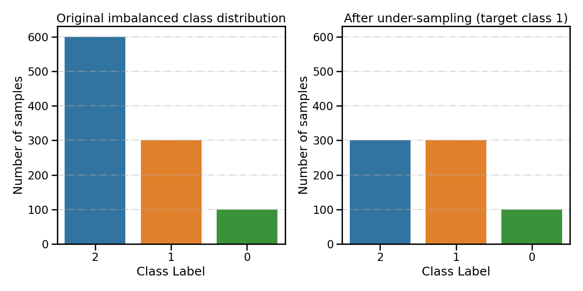
Specify the class targeted by the under-sampling
Set parameter ``target_label``: int All other classes that have more samples than the target class will be considered as majority classes. They will be under-sampled until the number of samples is equalized. The remaining minority classes (if any) will stay unchanged.
spe_clf.fit(X_train, y_train,
            target_label=1, # target class 1
            **fit_kwargs)

resampling_type='After under-sampling (target class 1)'
all_distribution[resampling_type] = spe_clf.target_distr_
plot_class_distribution_comparison(spe_clf, title2=resampling_type)
┏━━━━━━━━━━━━━┳━━━━━━━━━━━━━━━━━━━━━━━━━━┓
┃             ┃                          ┃
┃ #Estimators ┃    Class Distribution    ┃
┃             ┃                          ┃
┣━━━━━━━━━━━━━╋━━━━━━━━━━━━━━━━━━━━━━━━━━┫
┃      1      ┃ {0: 100, 1: 300, 2: 300} ┃
┣━━━━━━━━━━━━━╋━━━━━━━━━━━━━━━━━━━━━━━━━━┫
┃    final    ┃ {0: 100, 1: 300, 2: 300} ┃
┗━━━━━━━━━━━━━┻━━━━━━━━━━━━━━━━━━━━━━━━━━┛
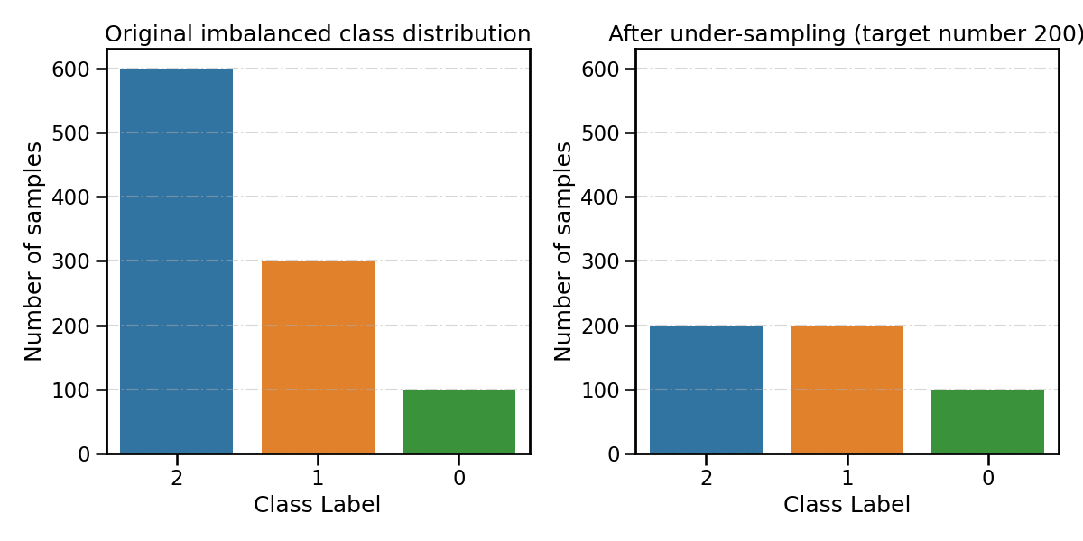
Specify the desired number of samples after under-sampling
Set parameter ``n_target_samples``: int or dict If int, all classes that have more than the n_target_samples samples will be under-sampled until the number of samples is equalized.
spe_clf.fit(X_train, y_train,
            n_target_samples=200, # target number of samples 200
            **fit_kwargs)

resampling_type='After under-sampling (target number 200)'
all_distribution[resampling_type] = spe_clf.target_distr_
plot_class_distribution_comparison(spe_clf, title2=resampling_type)
┏━━━━━━━━━━━━━┳━━━━━━━━━━━━━━━━━━━━━━━━━━┓
┃             ┃                          ┃
┃ #Estimators ┃    Class Distribution    ┃
┃             ┃                          ┃
┣━━━━━━━━━━━━━╋━━━━━━━━━━━━━━━━━━━━━━━━━━┫
┃      1      ┃ {0: 100, 1: 200, 2: 200} ┃
┣━━━━━━━━━━━━━╋━━━━━━━━━━━━━━━━━━━━━━━━━━┫
┃    final    ┃ {0: 100, 1: 200, 2: 200} ┃
┗━━━━━━━━━━━━━┻━━━━━━━━━━━━━━━━━━━━━━━━━━┛
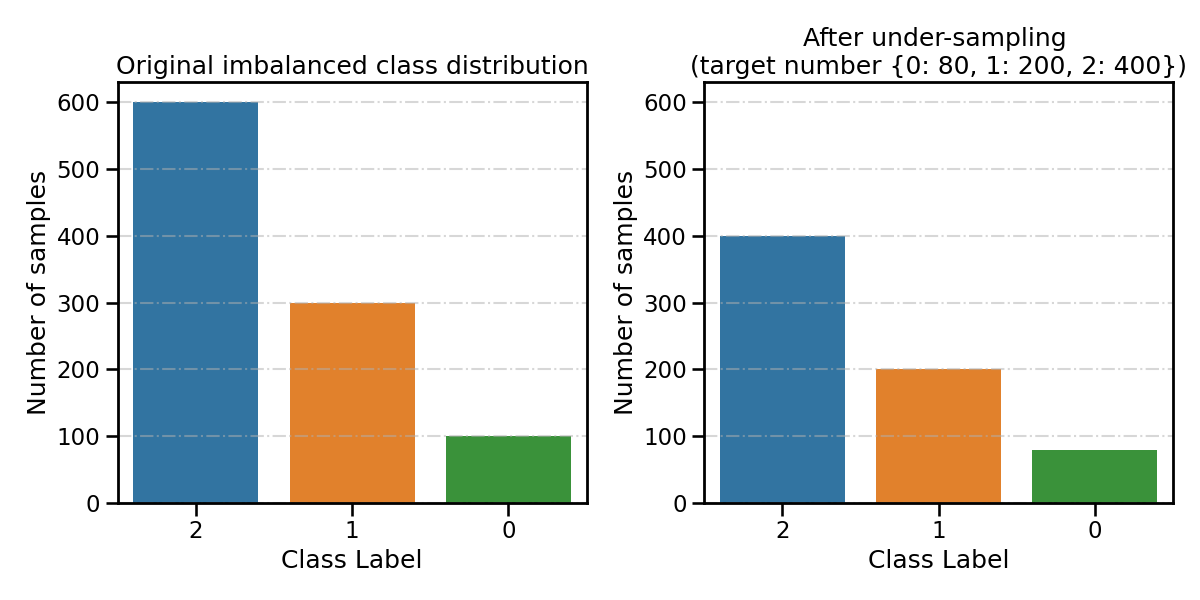
Specify the desired number of samples of each class after under-sampling
Set parameter ``n_target_samples``: int or dict If dict, the keys correspond to the targeted classes. The values correspond to the desired number of samples for each targeted class.
spe_clf.fit(X_train, y_train,
            n_target_samples={
                0: 80,
                1: 200,
                2: 400,
            }, # target number of samples
            **fit_kwargs)

resampling_type='After under-sampling \n(target number {0: 80, 1: 200, 2: 400})'
all_distribution[resampling_type] = spe_clf.target_distr_
plot_class_distribution_comparison(spe_clf, title2=resampling_type)
┏━━━━━━━━━━━━━┳━━━━━━━━━━━━━━━━━━━━━━━━━━┓
┃             ┃                          ┃
┃ #Estimators ┃    Class Distribution    ┃
┃             ┃                          ┃
┣━━━━━━━━━━━━━╋━━━━━━━━━━━━━━━━━━━━━━━━━━┫
┃      1      ┃ {0: 80, 1: 200, 2: 400}  ┃
┣━━━━━━━━━━━━━╋━━━━━━━━━━━━━━━━━━━━━━━━━━┫
┃    final    ┃ {0: 80, 1: 200, 2: 400}  ┃
┗━━━━━━━━━━━━━┻━━━━━━━━━━━━━━━━━━━━━━━━━━┛
Over-sampling
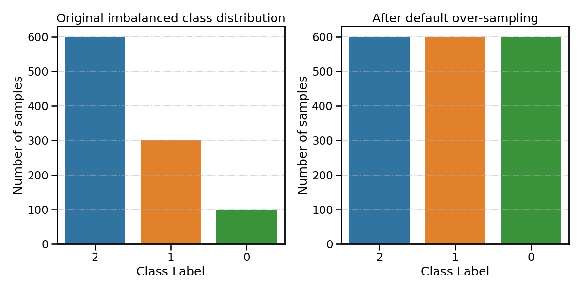
By default, over-sampling-based ensemble methods will consider the largest class as the majority class (class 2 with 600 samples). All other classes (class 0 and 1) will be considered as minority classes and will be over-sampled until the number of samples is equalized.
The over-sampling schedule can be customized in the same way as under-sampling.
Take SMOTEBoostClassifier as example
smoteboost_clf = imbens.ensemble.SMOTEBoostClassifier(**init_kwargs)
Train with the default under-sampling setting
smoteboost_clf.fit(X_train, y_train, **fit_kwargs)

all_distribution['Before over-sampling'] = smoteboost_clf.origin_distr_
resampling_type='After default over-sampling'
all_distribution[resampling_type] = smoteboost_clf.target_distr_
plot_class_distribution_comparison(smoteboost_clf, title2=resampling_type)
┏━━━━━━━━━━━━━┳━━━━━━━━━━━━━━━━━━━━━━━━━━┓
┃             ┃                          ┃
┃ #Estimators ┃    Class Distribution    ┃
┃             ┃                          ┃
┣━━━━━━━━━━━━━╋━━━━━━━━━━━━━━━━━━━━━━━━━━┫
┃      1      ┃ {0: 600, 1: 600, 2: 600} ┃
┣━━━━━━━━━━━━━╋━━━━━━━━━━━━━━━━━━━━━━━━━━┫
┃    final    ┃ {0: 600, 1: 600, 2: 600} ┃
┗━━━━━━━━━━━━━┻━━━━━━━━━━━━━━━━━━━━━━━━━━┛
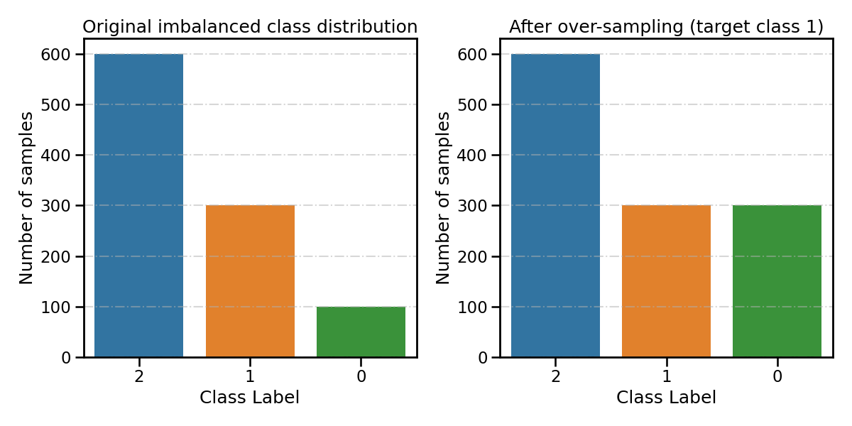
Specify the class targeted by the over-sampling
smoteboost_clf.fit(X_train, y_train,
                   target_label=1, # target class 1
                   **fit_kwargs)

resampling_type='After over-sampling (target class 1)'
all_distribution[resampling_type] = smoteboost_clf.target_distr_
plot_class_distribution_comparison(smoteboost_clf, title2=resampling_type)
┏━━━━━━━━━━━━━┳━━━━━━━━━━━━━━━━━━━━━━━━━━┓
┃             ┃                          ┃
┃ #Estimators ┃    Class Distribution    ┃
┃             ┃                          ┃
┣━━━━━━━━━━━━━╋━━━━━━━━━━━━━━━━━━━━━━━━━━┫
┃      1      ┃ {0: 300, 1: 300, 2: 600} ┃
┣━━━━━━━━━━━━━╋━━━━━━━━━━━━━━━━━━━━━━━━━━┫
┃    final    ┃ {0: 300, 1: 300, 2: 600} ┃
┗━━━━━━━━━━━━━┻━━━━━━━━━━━━━━━━━━━━━━━━━━┛
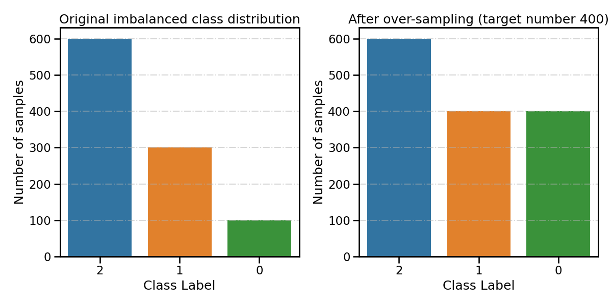
Specify the desired number of samples after over-sampling
smoteboost_clf.fit(X_train, y_train,
                   n_target_samples=400, # target number of samples 400
                   **fit_kwargs)

resampling_type='After over-sampling (target number 400)'
all_distribution[resampling_type] = smoteboost_clf.target_distr_
plot_class_distribution_comparison(smoteboost_clf, title2=resampling_type)
┏━━━━━━━━━━━━━┳━━━━━━━━━━━━━━━━━━━━━━━━━━┓
┃             ┃                          ┃
┃ #Estimators ┃    Class Distribution    ┃
┃             ┃                          ┃
┣━━━━━━━━━━━━━╋━━━━━━━━━━━━━━━━━━━━━━━━━━┫
┃      1      ┃ {0: 400, 1: 400, 2: 600} ┃
┣━━━━━━━━━━━━━╋━━━━━━━━━━━━━━━━━━━━━━━━━━┫
┃    final    ┃ {0: 400, 1: 400, 2: 600} ┃
┗━━━━━━━━━━━━━┻━━━━━━━━━━━━━━━━━━━━━━━━━━┛
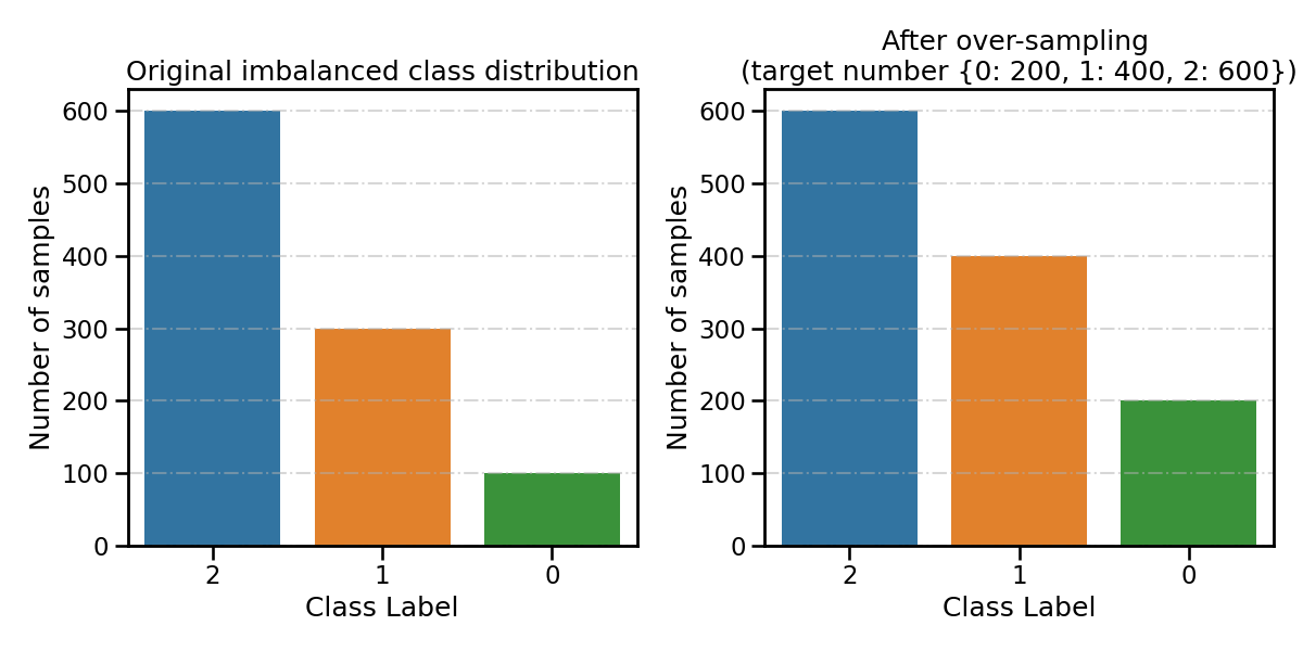
Specify the desired number of samples of each class after over-sampling
smoteboost_clf.fit(X_train, y_train,
                   n_target_samples={
                       0: 200,
                       1: 400,
                       2: 600,
                   }, # target number of samples
                   **fit_kwargs)

resampling_type='After over-sampling \n(target number {0: 200, 1: 400, 2: 600})'
all_distribution[resampling_type] = smoteboost_clf.target_distr_
plot_class_distribution_comparison(smoteboost_clf, title2=resampling_type)
┏━━━━━━━━━━━━━┳━━━━━━━━━━━━━━━━━━━━━━━━━━┓
┃             ┃                          ┃
┃ #Estimators ┃    Class Distribution    ┃
┃             ┃                          ┃
┣━━━━━━━━━━━━━╋━━━━━━━━━━━━━━━━━━━━━━━━━━┫
┃      1      ┃ {0: 200, 1: 400, 2: 600} ┃
┣━━━━━━━━━━━━━╋━━━━━━━━━━━━━━━━━━━━━━━━━━┫
┃    final    ┃ {0: 200, 1: 400, 2: 600} ┃
┗━━━━━━━━━━━━━┻━━━━━━━━━━━━━━━━━━━━━━━━━━┛
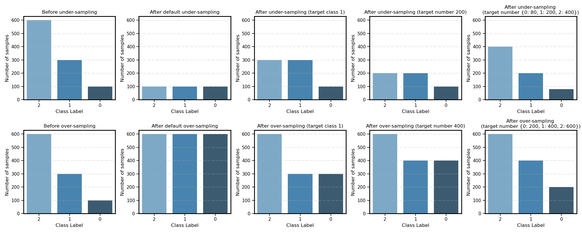
Visualize different resampling target
sns.set_context('notebook')
fig, axes = plt.subplots(2, 5, figsize=(20, 8))
for ax, title in zip(axes.flatten(), list(all_distribution.keys())):
    plot_class_distribution(all_distribution[title], ax=ax, palette="Blues_d")
    ax.set(ylim=ylim, title=title)
fig.tight_layout()
Total running time of the script: ( 0 minutes 1.035 seconds)