Classify class-imbalanced hand-written digits

This example shows how imbalanced-ensemble can be used to cooperate with scikit-learn base classifier and recognize images of hand-written digits, from 0-9.

This example uses:

• imbens.ensemble.SelfPacedEnsembleClassifier

• imbens.visualizer.ImbalancedEnsembleVisualizer

# Adapted from sklearn
# Author: Zhining Liu <zhining.liu@outlook.com>
#         Gael Varoquaux <gael dot varoquaux at normalesup dot org>
# License: BSD 3 clause

print(__doc__)

# Import imbalanced-ensemble
import imbens

# Import utilities
import sklearn
from sklearn.model_selection import train_test_split
from imbens.datasets import make_imbalance
from imbens.utils._plot import plot_2Dprojection_and_cardinality
import matplotlib.pyplot as plt

RANDOM_STATE = 42

Digits dataset

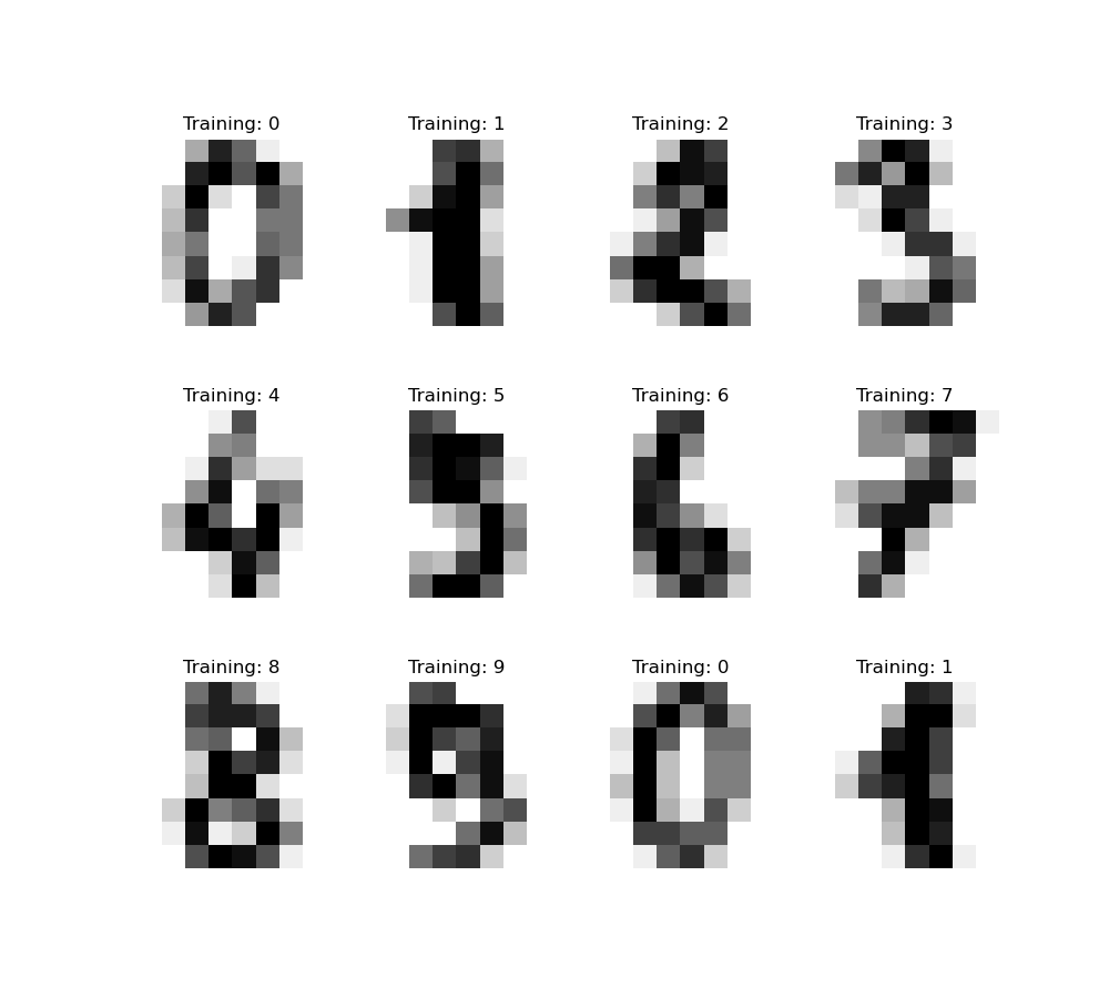
The digits dataset consists of 8x8 pixel images of digits. The images attribute of the dataset stores 8x8 arrays of grayscale values for each image. We will use these arrays to visualize the first 4 images. The target attribute of the dataset stores the digit each image represents and this is included in the title of the 4 plots below.

To apply a classifier on this data, we need to flatten the images, turning each 2-D array of grayscale values from shape (8, 8) into shape (64,). Subsequently, the entire dataset will be of shape (n_samples, n_features), where n_samples is the number of images and n_features is the total number of pixels in each image.

digits = sklearn.datasets.load_digits()

# flatten the images
n_samples = len(digits.images)
X, y = digits.images.reshape((n_samples, -1)), digits.target

_, axes = plt.subplots(nrows=3, ncols=4, figsize=(10, 9))
for ax, image, label in zip(axes.flatten(), digits.images, digits.target):
    ax.set_axis_off()
    ax.imshow(image, cmap=plt.cm.gray_r, interpolation='nearest')
    ax.set_title('Training: %i' % label)

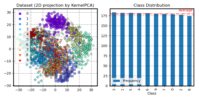
The original digits dataset

fig = plot_2Dprojection_and_cardinality(X, y, figsize=(8, 4))

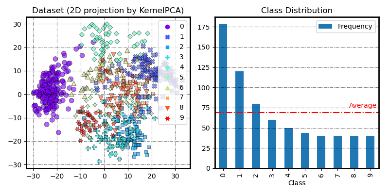
Make class-imbalanced digits dataset

imbalance_distr = {0: 178, 1: 120, 2: 80, 3: 60, 4: 50, 5: 44, 6: 40, 7: 40, 8: 40, 9: 40}

X, y = make_imbalance(X, y, sampling_strategy=imbalance_distr, random_state=RANDOM_STATE)

fig = plot_2Dprojection_and_cardinality(X, y, figsize=(8, 4))

Classification

We split the data into train and test subsets and fit a SelfPacedEnsembleClassifier (with support vector machine as base classifier) on the train samples. The fitted classifier can subsequently be used to predict the value of the digit for the samples in the test subset.

# Split data into 50% train and 50% test subsets
X_train, X_test, y_train, y_test = train_test_split(
    X, y, test_size=0.5, shuffle=True, stratify=y, random_state=0)

# Create a classifier: a SPE with support vector base classifier
base_clf = sklearn.svm.SVC(gamma=0.001, probability=True)
clf = imbens.ensemble.SelfPacedEnsembleClassifier(
    n_estimators=5, estimator=base_clf,
)

# Learn the digits on the train subset
clf.fit(X_train, y_train)

# Predict the value of the digit on the test subset
predicted = clf.predict(X_test)

sklearn.metrics.classification_report builds a text report showing the main classification metrics.

print(f"Classification report for classifier {clf}:\n"
      f"{sklearn.metrics.classification_report(y_test, predicted)}\n")

Classification report for classifier SelfPacedEnsembleClassifier(estimator=SVC(gamma=0.001, probability=True),
                            n_estimators=5,
                            random_state=RandomState(MT19937) at 0x247543B9540):
              precision    recall  f1-score   support

           0       1.00      1.00      1.00        89
           1       0.97      1.00      0.98        60
           2       1.00      0.97      0.99        40
           3       0.96      0.90      0.93        30
           4       1.00      0.96      0.98        25
           5       0.91      0.95      0.93        22
           6       1.00      1.00      1.00        20
           7       0.90      0.95      0.93        20
           8       0.90      0.95      0.93        20
           9       0.89      0.85      0.87        20

    accuracy                           0.97       346
   macro avg       0.95      0.95      0.95       346
weighted avg       0.97      0.97      0.97       346

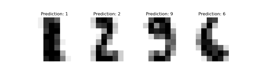
Below we visualize the first 4 test samples and show their predicted digit value in the title.

_, axes = plt.subplots(nrows=1, ncols=4, figsize=(10, 3))
for ax, image, prediction in zip(axes, X_test, predicted):
    ax.set_axis_off()
    image = image.reshape(8, 8)
    ax.imshow(image, cmap=plt.cm.gray_r, interpolation='nearest')
    ax.set_title(f'Prediction: {prediction}')

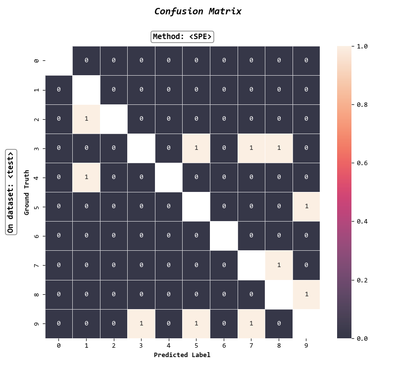
We can also plot a confusion matrix of the true digit values and the predicted digit values using the ImbalancedEnsembleVisualizer.

visualizer = imbens.visualizer.ImbalancedEnsembleVisualizer(
    eval_datasets = {
        'test' : (X_test, y_test),
    },
).fit({'SPE': clf})

fig, axes = visualizer.confusion_matrix_heatmap(
    sub_figsize=(8, 7),
    false_pred_only=True,
)

  0%|                                                                                                                                                                                                                                                                               | 0/5 [00:00<?, ?it/s]
Visualizer evaluating model SPE on dataset test ::   0%|                                                                                                                                                                                                                            | 0/5 [00:00<?, ?it/s]
Visualizer evaluating model SPE on dataset test :: 100%|####################################################################################################################################################################################################################| 5/5 [00:00<00:00, 76.76it/s]
Visualizer computing confusion matrices. Finished!