Note
Go to the end to download the full example code.
Use dynamic resampling schedule
This example demonstrates how to customize the sampling schedule to achieve dynamic resampling. This can be easily done by setting the “balancing_schedule” parameter when calling the “fit()” method.
Note that this feature only applies to resampling-based ensemble classifiers that are iteratively trained.
This example uses:
# Authors: Zhining Liu <zhining.liu@outlook.com>
# License: MIT
print(__doc__)

# Import imbalanced-ensemble
import imbens

# Import utilities
import math
import sklearn
from sklearn.datasets import make_classification
from sklearn.model_selection import train_test_split
from imbens.ensemble.base import sort_dict_by_key
from collections import Counter

RANDOM_STATE = 42

init_kwargs = {
    'n_estimators': 5,
    'random_state': RANDOM_STATE,
}
fit_kwargs = {
    'train_verbose': {
        'granularity': 1,
        'print_metrics': False,
    },
}

# sphinx_gallery_thumbnail_number = 3
Prepare data
Make a toy 3-class imbalanced classification task.
# make dataset
X, y = make_classification(
    n_classes=3,
    class_sep=2,
    weights=[0.1, 0.3, 0.6],
    n_informative=3,
    n_redundant=1,
    flip_y=0,
    n_features=20,
    n_clusters_per_class=2,
    n_samples=2000,
    random_state=0,
)

# train valid split
X_train, X_valid, y_train, y_valid = train_test_split(
    X, y, test_size=0.5, stratify=y, random_state=RANDOM_STATE
)
Print the original class/marginal distribution P(Y) of the training data
print('Original training dataset distribution %s' % sort_dict_by_key(Counter(y_train)))
Original training dataset distribution {np.int64(0): 100, np.int64(1): 300, np.int64(2): 600}
Uniform under-sampling
By default, under-sampling-based ensemble methods will consider the smallest class as the minority class (class 0 with 100 samples). All other classes (class 1 and 2) will be considered as majority classes and will be under-sampled until the number of samples is equalized.
Take SelfPacedEnsembleClassifier as example
spe_clf = imbens.ensemble.SelfPacedEnsembleClassifier(**init_kwargs)
Train with the default under-sampling setting
spe_clf.fit(X_train, y_train, **fit_kwargs)
┏━━━━━━━━━━━━━┳━━━━━━━━━━━━━━━━━━━━━━━━━━━━━━━━━━━━━━━━━━━━━━━━━━━━━━━━┓
┃             ┃                                                        ┃
┃ #Estimators ┃                   Class Distribution                   ┃
┃             ┃                                                        ┃
┣━━━━━━━━━━━━━╋━━━━━━━━━━━━━━━━━━━━━━━━━━━━━━━━━━━━━━━━━━━━━━━━━━━━━━━━┫
┃      1      ┃ {np.int64(0): 100, np.int64(1): 100, np.int64(2): 100} ┃
┃      2      ┃ {np.int64(0): 100, np.int64(1): 100, np.int64(2): 100} ┃
┃      3      ┃ {np.int64(0): 100, np.int64(1): 100, np.int64(2): 100} ┃
┃      4      ┃ {np.int64(0): 100, np.int64(1): 100, np.int64(2): 100} ┃
┃      5      ┃ {np.int64(0): 100, np.int64(1): 100, np.int64(2): 100} ┃
┣━━━━━━━━━━━━━╋━━━━━━━━━━━━━━━━━━━━━━━━━━━━━━━━━━━━━━━━━━━━━━━━━━━━━━━━┫
┃    final    ┃ {np.int64(0): 100, np.int64(1): 100, np.int64(2): 100} ┃
┗━━━━━━━━━━━━━┻━━━━━━━━━━━━━━━━━━━━━━━━━━━━━━━━━━━━━━━━━━━━━━━━━━━━━━━━┛
Progressive under-sampling
The resample class distributions are progressive interpolation between the original and the target class distribution. Example: For a class \(c\), say the number of samples is \(N_{c}\) and the target number of samples is \(N'_{c}\). Suppose that we are training the \(t\)-th base estimator of a \(T\)-estimator ensemble, then we expect to get \((1-\frac{t}{T}) \cdot N_{c} + \frac{t}{T} \cdot N'_{c}\) samples after resampling;
Train with progressive under-sampling schedule
spe_clf.fit(
    X_train,
    y_train,
    balancing_schedule='progressive',  # Progeressive under-sampling
    **fit_kwargs,
)
┏━━━━━━━━━━━━━┳━━━━━━━━━━━━━━━━━━━━━━━━━━━━━━━━━━━━━━━━━━━━━━━━━━━━━━━━┓
┃             ┃                                                        ┃
┃ #Estimators ┃                   Class Distribution                   ┃
┃             ┃                                                        ┃
┣━━━━━━━━━━━━━╋━━━━━━━━━━━━━━━━━━━━━━━━━━━━━━━━━━━━━━━━━━━━━━━━━━━━━━━━┫
┃      1      ┃ {np.int64(0): 100, np.int64(1): 300, np.int64(2): 600} ┃
┃      2      ┃ {np.int64(0): 100, np.int64(1): 250, np.int64(2): 475} ┃
┃      3      ┃ {np.int64(0): 100, np.int64(1): 200, np.int64(2): 350} ┃
┃      4      ┃ {np.int64(0): 100, np.int64(1): 150, np.int64(2): 225} ┃
┃      5      ┃ {np.int64(0): 100, np.int64(1): 100, np.int64(2): 100} ┃
┣━━━━━━━━━━━━━╋━━━━━━━━━━━━━━━━━━━━━━━━━━━━━━━━━━━━━━━━━━━━━━━━━━━━━━━━┫
┃    final    ┃ {np.int64(0): 100, np.int64(1): 100, np.int64(2): 100} ┃
┗━━━━━━━━━━━━━┻━━━━━━━━━━━━━━━━━━━━━━━━━━━━━━━━━━━━━━━━━━━━━━━━━━━━━━━━┛
Define your own resampling schedule.
Your schedule function should take 4 positional arguments with order ('origin_distr':
dict, 'target_distr': dict, 'i_estimator': int, 'total_estimator':
int), and returns a 'result_distr': dict. For all parameters of type dict,
the keys of type int correspond to the targeted classes, and the values of type str
correspond to the (desired) number of samples for each class.
Train with user-defined dummy resampling schedule
def my_dummy_schedule(
    origin_distr: dict, target_distr: dict, i_estimator: int, total_estimator: int
):
    '''A dummy resampling schedule'''
    return origin_distr


spe_clf.fit(
    X_train,
    y_train,
    balancing_schedule=my_dummy_schedule,  # Use your progressive resampling schedule
    **fit_kwargs,
)
┏━━━━━━━━━━━━━┳━━━━━━━━━━━━━━━━━━━━━━━━━━━━━━━━━━━━━━━━━━━━━━━━━━━━━━━━┓
┃             ┃                                                        ┃
┃ #Estimators ┃                   Class Distribution                   ┃
┃             ┃                                                        ┃
┣━━━━━━━━━━━━━╋━━━━━━━━━━━━━━━━━━━━━━━━━━━━━━━━━━━━━━━━━━━━━━━━━━━━━━━━┫
┃      1      ┃ {np.int64(0): 100, np.int64(1): 300, np.int64(2): 600} ┃
┃      2      ┃ {np.int64(0): 100, np.int64(1): 300, np.int64(2): 600} ┃
┃      3      ┃ {np.int64(0): 100, np.int64(1): 300, np.int64(2): 600} ┃
┃      4      ┃ {np.int64(0): 100, np.int64(1): 300, np.int64(2): 600} ┃
┃      5      ┃ {np.int64(0): 100, np.int64(1): 300, np.int64(2): 600} ┃
┣━━━━━━━━━━━━━╋━━━━━━━━━━━━━━━━━━━━━━━━━━━━━━━━━━━━━━━━━━━━━━━━━━━━━━━━┫
┃    final    ┃ {np.int64(0): 100, np.int64(1): 300, np.int64(2): 600} ┃
┗━━━━━━━━━━━━━┻━━━━━━━━━━━━━━━━━━━━━━━━━━━━━━━━━━━━━━━━━━━━━━━━━━━━━━━━┛
Train with user-defined progressive resampling schedule
def my_progressive_schedule(
    origin_distr: dict, target_distr: dict, i_estimator: int, total_estimator: int
):
    '''A user-defined progressive resampling schedule'''
    # compute training progress
    p = i_estimator / (total_estimator - 1) if total_estimator >= 1 else 1
    result_distr = {}
    # compute expected number of samples for each class
    for label in origin_distr.keys():
        result_distr[label] = math.ceil(
            origin_distr[label] * (1 - p)
            + target_distr[label] * p
            - 1e-10  # for numerical stability
        )
    return result_distr


spe_clf.fit(
    X_train,
    y_train,
    balancing_schedule=my_progressive_schedule,  # Use your progressive resampling schedule
    **fit_kwargs,
)
┏━━━━━━━━━━━━━┳━━━━━━━━━━━━━━━━━━━━━━━━━━━━━━━━━━━━━━━━━━━━━━━━━━━━━━━━┓
┃             ┃                                                        ┃
┃ #Estimators ┃                   Class Distribution                   ┃
┃             ┃                                                        ┃
┣━━━━━━━━━━━━━╋━━━━━━━━━━━━━━━━━━━━━━━━━━━━━━━━━━━━━━━━━━━━━━━━━━━━━━━━┫
┃      1      ┃ {np.int64(0): 100, np.int64(1): 300, np.int64(2): 600} ┃
┃      2      ┃ {np.int64(0): 100, np.int64(1): 250, np.int64(2): 475} ┃
┃      3      ┃ {np.int64(0): 100, np.int64(1): 200, np.int64(2): 350} ┃
┃      4      ┃ {np.int64(0): 100, np.int64(1): 150, np.int64(2): 225} ┃
┃      5      ┃ {np.int64(0): 100, np.int64(1): 100, np.int64(2): 100} ┃
┣━━━━━━━━━━━━━╋━━━━━━━━━━━━━━━━━━━━━━━━━━━━━━━━━━━━━━━━━━━━━━━━━━━━━━━━┫
┃    final    ┃ {np.int64(0): 100, np.int64(1): 100, np.int64(2): 100} ┃
┗━━━━━━━━━━━━━┻━━━━━━━━━━━━━━━━━━━━━━━━━━━━━━━━━━━━━━━━━━━━━━━━━━━━━━━━┛
Over-sampling
By default, over-sampling-based ensemble methods will consider the largest class as the majority class (class 2 with 600 samples). All other classes (class 0 and 1) will be considered as minority classes and will be over-sampled until the number of samples is equalized.
The over-sampling schedule can be customized in the same way as under-sampling.
Take SMOTEBoostClassifier as example
smoteboost_clf = imbens.ensemble.SMOTEBoostClassifier(**init_kwargs)
Train with the default over-sampling setting
smoteboost_clf.fit(X_train, y_train, **fit_kwargs)
┏━━━━━━━━━━━━━┳━━━━━━━━━━━━━━━━━━━━━━━━━━━━━━━━━━━━━━━━━━━━━━━━━━━━━━━━┓
┃             ┃                                                        ┃
┃ #Estimators ┃                   Class Distribution                   ┃
┃             ┃                                                        ┃
┣━━━━━━━━━━━━━╋━━━━━━━━━━━━━━━━━━━━━━━━━━━━━━━━━━━━━━━━━━━━━━━━━━━━━━━━┫
┃      1      ┃ {np.int64(0): 600, np.int64(1): 600, np.int64(2): 600} ┃
┃      2      ┃ {np.int64(0): 600, np.int64(1): 600, np.int64(2): 600} ┃
┃      3      ┃ {np.int64(0): 600, np.int64(1): 600, np.int64(2): 600} ┃
┃      4      ┃ {np.int64(0): 600, np.int64(1): 600, np.int64(2): 600} ┃
┃      5      ┃ {np.int64(0): 600, np.int64(1): 600, np.int64(2): 600} ┃
┣━━━━━━━━━━━━━╋━━━━━━━━━━━━━━━━━━━━━━━━━━━━━━━━━━━━━━━━━━━━━━━━━━━━━━━━┫
┃    final    ┃ {np.int64(0): 600, np.int64(1): 600, np.int64(2): 600} ┃
┗━━━━━━━━━━━━━┻━━━━━━━━━━━━━━━━━━━━━━━━━━━━━━━━━━━━━━━━━━━━━━━━━━━━━━━━┛
Train with progressive over-sampling schedule
smoteboost_clf.fit(X_train, y_train, balancing_schedule='progressive', **fit_kwargs)
┏━━━━━━━━━━━━━┳━━━━━━━━━━━━━━━━━━━━━━━━━━━━━━━━━━━━━━━━━━━━━━━━━━━━━━━━┓
┃             ┃                                                        ┃
┃ #Estimators ┃                   Class Distribution                   ┃
┃             ┃                                                        ┃
┣━━━━━━━━━━━━━╋━━━━━━━━━━━━━━━━━━━━━━━━━━━━━━━━━━━━━━━━━━━━━━━━━━━━━━━━┫
┃      1      ┃ {np.int64(0): 100, np.int64(1): 300, np.int64(2): 600} ┃
┃      2      ┃ {np.int64(0): 225, np.int64(1): 375, np.int64(2): 600} ┃
┃      3      ┃ {np.int64(0): 350, np.int64(1): 450, np.int64(2): 600} ┃
┃      4      ┃ {np.int64(0): 475, np.int64(1): 525, np.int64(2): 600} ┃
┃      5      ┃ {np.int64(0): 600, np.int64(1): 600, np.int64(2): 600} ┃
┣━━━━━━━━━━━━━╋━━━━━━━━━━━━━━━━━━━━━━━━━━━━━━━━━━━━━━━━━━━━━━━━━━━━━━━━┫
┃    final    ┃ {np.int64(0): 600, np.int64(1): 600, np.int64(2): 600} ┃
┗━━━━━━━━━━━━━┻━━━━━━━━━━━━━━━━━━━━━━━━━━━━━━━━━━━━━━━━━━━━━━━━━━━━━━━━┛
Train with user-defined dummy resampling schedule
smoteboost_clf.fit(X_train, y_train, balancing_schedule=my_dummy_schedule, **fit_kwargs)
┏━━━━━━━━━━━━━┳━━━━━━━━━━━━━━━━━━━━━━━━━━━━━━━━━━━━━━━━━━━━━━━━━━━━━━━━┓
┃             ┃                                                        ┃
┃ #Estimators ┃                   Class Distribution                   ┃
┃             ┃                                                        ┃
┣━━━━━━━━━━━━━╋━━━━━━━━━━━━━━━━━━━━━━━━━━━━━━━━━━━━━━━━━━━━━━━━━━━━━━━━┫
┃      1      ┃ {np.int64(0): 100, np.int64(1): 300, np.int64(2): 600} ┃
┃      2      ┃ {np.int64(0): 100, np.int64(1): 300, np.int64(2): 600} ┃
┃      3      ┃ {np.int64(0): 100, np.int64(1): 300, np.int64(2): 600} ┃
┃      4      ┃ {np.int64(0): 100, np.int64(1): 300, np.int64(2): 600} ┃
┃      5      ┃ {np.int64(0): 100, np.int64(1): 300, np.int64(2): 600} ┃
┣━━━━━━━━━━━━━╋━━━━━━━━━━━━━━━━━━━━━━━━━━━━━━━━━━━━━━━━━━━━━━━━━━━━━━━━┫
┃    final    ┃ {np.int64(0): 100, np.int64(1): 300, np.int64(2): 600} ┃
┗━━━━━━━━━━━━━┻━━━━━━━━━━━━━━━━━━━━━━━━━━━━━━━━━━━━━━━━━━━━━━━━━━━━━━━━┛
Train with user-defined progressive resampling schedule
smoteboost_clf.fit(
    X_train, y_train, balancing_schedule=my_progressive_schedule, **fit_kwargs
)
┏━━━━━━━━━━━━━┳━━━━━━━━━━━━━━━━━━━━━━━━━━━━━━━━━━━━━━━━━━━━━━━━━━━━━━━━┓
┃             ┃                                                        ┃
┃ #Estimators ┃                   Class Distribution                   ┃
┃             ┃                                                        ┃
┣━━━━━━━━━━━━━╋━━━━━━━━━━━━━━━━━━━━━━━━━━━━━━━━━━━━━━━━━━━━━━━━━━━━━━━━┫
┃      1      ┃ {np.int64(0): 100, np.int64(1): 300, np.int64(2): 600} ┃
┃      2      ┃ {np.int64(0): 225, np.int64(1): 375, np.int64(2): 600} ┃
┃      3      ┃ {np.int64(0): 350, np.int64(1): 450, np.int64(2): 600} ┃
┃      4      ┃ {np.int64(0): 475, np.int64(1): 525, np.int64(2): 600} ┃
┃      5      ┃ {np.int64(0): 600, np.int64(1): 600, np.int64(2): 600} ┃
┣━━━━━━━━━━━━━╋━━━━━━━━━━━━━━━━━━━━━━━━━━━━━━━━━━━━━━━━━━━━━━━━━━━━━━━━┫
┃    final    ┃ {np.int64(0): 600, np.int64(1): 600, np.int64(2): 600} ┃
┗━━━━━━━━━━━━━┻━━━━━━━━━━━━━━━━━━━━━━━━━━━━━━━━━━━━━━━━━━━━━━━━━━━━━━━━┛
Visualize different resampling schedule
Implement some plot utilities
import matplotlib.pyplot as plt
import seaborn as sns
from imbens.utils._plot import set_ax_border

ylim = (0, 630)


def plot_class_distribution(
    distr: dict,
    xlabel: str = 'Class Label',
    ylabel: str = 'Number of samples',
    **kwargs,
):
    distr = dict(sorted(distr.items(), key=lambda k: k[0], reverse=True))
    ax = sns.barplot(
        x=list(distr.keys()), y=list(distr.values()), order=list(distr.keys()), **kwargs
    )
    set_ax_border(ax)
    ax.grid(axis='y', alpha=0.5, ls='-.')
    ax.set_xlabel(xlabel)
    ax.set_ylabel(ylabel)
    return ax
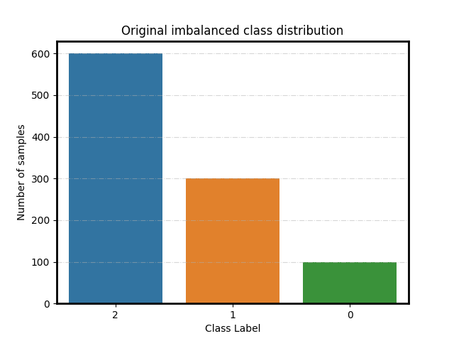
Original class distribution
ax = plot_class_distribution(spe_clf.origin_distr_)
ax.set_title('Original imbalanced class distribution')
Text(0.5, 1.0, 'Original imbalanced class distribution')
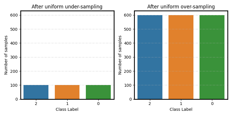
Uniform under/over-sampling
fig, (ax1, ax2) = plt.subplots(1, 2, figsize=(8, 4))

plot_class_distribution(spe_clf.target_distr_, ax=ax1)
ax1.set(ylim=ylim, title='After uniform under-sampling')
plot_class_distribution(smoteboost_clf.target_distr_, ax=ax2)
ax2.set(ylim=ylim, title='After uniform over-sampling')

fig.tight_layout()
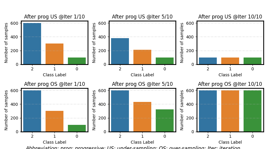
Progressive under/over-sampling
from imbens.utils._validation_param import _progressive_schedule

N = 10
i_estimators = [0, 4, 9]
origin_distr = sort_dict_by_key(Counter(y_train))
under_distr = spe_clf.target_distr_
over_distr = smoteboost_clf.target_distr_

fig, axes = plt.subplots(2, 3, figsize=(9, 5))

# Progressive under-sampling
for ax, i in zip(axes[0], i_estimators):
    resample_distr = _progressive_schedule(origin_distr, under_distr, i, N)
    plot_class_distribution(resample_distr, ax=ax)
    ax.set(ylim=ylim, title=f'After prog US @Iter {i+1}/{N}')

# Progressive over-sampling
for ax, i in zip(axes[1], i_estimators):
    resample_distr = _progressive_schedule(origin_distr, over_distr, i, N)
    plot_class_distribution(resample_distr, ax=ax)
    ax.set(ylim=ylim, title=f'After prog OS @Iter {i+1}/{N}')

fig.suptitle(
    "Abbreviation: prog: progressive; US: under-sampling; OS: over-sampling; Iter: iteration.",
    y=0.02,
    style='italic',
)
fig.tight_layout()
Total running time of the script: (0 minutes 1.116 seconds)