Customize cost matrix

This example demonstrates how to customize the cost matrix of cost-sensitive ensemble methods.

This example uses:

• imbens.ensemble.AdaCostClassifier

# Authors: Zhining Liu <zhining.liu@outlook.com>
# License: MIT

print(__doc__)

# Import imbalanced-ensemble
import imbens

# Import utilities
import numpy as np
import sklearn
from sklearn.datasets import make_classification
from sklearn.model_selection import train_test_split
from imbens.ensemble.base import sort_dict_by_key
from collections import Counter

# Import plot utilities
import matplotlib.pyplot as plt
import seaborn as sns

sns.set_context('talk')

RANDOM_STATE = 42

init_kwargs = {
    'n_estimators': 5,
    'random_state': RANDOM_STATE,
}

# sphinx_gallery_thumbnail_number = -2

Prepare data

Make a toy 3-class imbalanced classification task.

# make dataset
X, y = make_classification(
    n_classes=3,
    class_sep=2,
    weights=[0.1, 0.3, 0.6],
    n_informative=3,
    n_redundant=1,
    flip_y=0,
    n_features=20,
    n_clusters_per_class=2,
    n_samples=2000,
    random_state=0,
)

# train valid split
X_train, X_valid, y_train, y_valid = train_test_split(
    X, y, test_size=0.5, stratify=y, random_state=RANDOM_STATE
)

# Print class distribution
print('Training dataset distribution    %s' % sort_dict_by_key(Counter(y_train)))
print('Validation dataset distribution  %s' % sort_dict_by_key(Counter(y_valid)))

Training dataset distribution    {0: 100, 1: 300, 2: 600}
Validation dataset distribution  {0: 100, 1: 300, 2: 600}

Implement some plot utilities

cost_matrices = {}


def plot_cost_matrix(cost_matrix, title: str, **kwargs):
    ax = sns.heatmap(data=cost_matrix, **kwargs)
    ax.set_ylabel("Predicted Label")
    ax.set_xlabel("Ground Truth")
    ax.set_title(title)

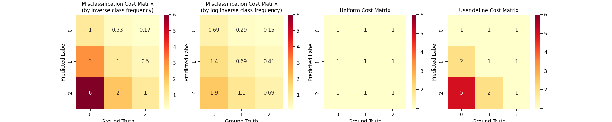
Default Cost Matrix

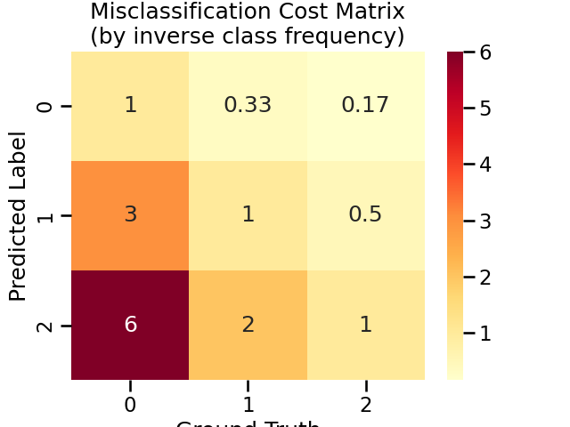
By default, cost-sensitive ensemble methods will set misclassification cost by inverse class frequency.

You can access the ``clf.cost_matrix_`` attribute (``clf`` is a fitted cost-sensitive ensemble classifier) to view the cost matrix used for training. The rows represent the predicted class and columns represent the actual class. Note that the order of the classes corresponds to that in the attribute clf.classes_.

Take AdaCostClassifier as example

adacost_clf = imbens.ensemble.AdaCostClassifier(**init_kwargs)

Train with the default cost matrix setting

adacost_clf.fit(X_train, y_train)

adacost_clf.cost_matrix_

array([[1.        , 0.33333333, 0.16666667],
       [3.        , 1.        , 0.5       ],
       [6.        , 2.        , 1.        ]])

Visualize the default cost matrix

title = "Misclassification Cost Matrix\n(by inverse class frequency)"
cost_matrices[title] = adacost_clf.cost_matrix_
plot_cost_matrix(adacost_clf.cost_matrix_, title, annot=True, cmap='YlOrRd', vmax=6)

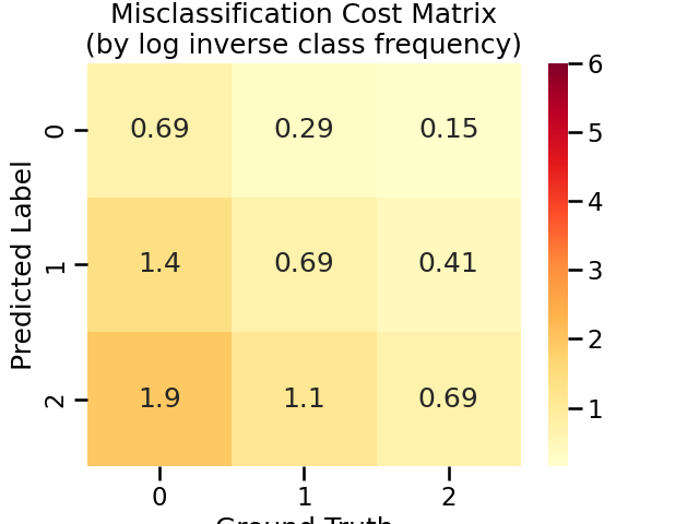
log1p-inverse Cost Matrix

You can set misclassification cost by log inverse class frequency by set cost_matrix = 'log1p-inverse'. This usually leads to a “softer” cost matrix, that is, less penalty for misclassification of minority class samples into the majority class.

adacost_clf.fit(
    X_train,
    y_train,
    cost_matrix='log1p-inverse',  # set cost matrix by log inverse class frequency
)

adacost_clf.cost_matrix_

array([[0.69314718, 0.28768207, 0.15415068],
       [1.38629436, 0.69314718, 0.40546511],
       [1.94591015, 1.09861229, 0.69314718]])

Visualize the log1p-inverse cost matrix

title = "Misclassification Cost Matrix\n(by log inverse class frequency)"
cost_matrices[title] = adacost_clf.cost_matrix_
plot_cost_matrix(adacost_clf.cost_matrix_, title, annot=True, cmap='YlOrRd', vmax=6)

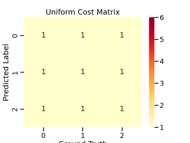
Use Uniform Cost Matrix

You can set misclassification cost by log inverse class frequency by set cost_matrix = 'uniform'.

# Note that this will set all misclassification cost to be equal, i.e., model will not be cost-sensitive.

adacost_clf.fit(
    X_train,
    y_train,
    cost_matrix='uniform',  # set cost matrix to be uniform
)

adacost_clf.cost_matrix_

array([[1., 1., 1.],
       [1., 1., 1.],
       [1., 1., 1.]])

Visualize the uniform cost matrix

title = "Uniform Cost Matrix"
cost_matrices[title] = adacost_clf.cost_matrix_
plot_cost_matrix(adacost_clf.cost_matrix_, title, annot=True, cmap='YlOrRd', vmax=6)

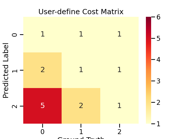
Use Your Own Cost Matrix

You can also set misclassification cost by explicitly passing your cost matrix to cost_matrix.

Your cost matrix must be a numpy.2darray of shape (n_classes, n_classes), the rows represent the predicted class and columns represent the actual class. Thus the value at \(i\)-th row \(j\)-th column represents the cost of classifying a sample from class \(j\) to class \(i\).

# set your own cost matrix
my_cost_matrix = [
    [1, 1, 1],
    [2, 1, 1],
    [5, 2, 1],
]

adacost_clf.fit(
    X_train,
    y_train,
    cost_matrix=my_cost_matrix,  # use your cost matrix
)

adacost_clf.cost_matrix_

array([[1, 1, 1],
       [2, 1, 1],
       [5, 2, 1]])

Visualize the user-define cost matrix

title = "User-define Cost Matrix"
cost_matrices[title] = adacost_clf.cost_matrix_
plot_cost_matrix(adacost_clf.cost_matrix_, title, annot=True, cmap='YlOrRd', vmax=6)

Visualize All Used Cost Matrices

sns.set_context('notebook')
fig, axes = plt.subplots(1, 4, figsize=(20, 4))
for ax, title in zip(axes, cost_matrices.keys()):
    plot_cost_matrix(
        cost_matrices[title], title, annot=True, cmap='YlOrRd', vmax=6, ax=ax
    )