ImbalancedEnsembleVisualizer
- class imbens.visualizer.ImbalancedEnsembleVisualizer(eval_metrics: dict = None, eval_datasets: dict = None)[source]
A visualizer, providing several utilities to visualize:
the model performance curve with respect to the number of base estimators / training samples, could be grouped by method, evaluation dataset, or both;
the confusion matrix of the model prediction.
This visualization tool can be used to:
provide further information about the training process (for iteratively trained ensemble) of a single ensemble model;
or to compare the performance of multiple different ensemble models in an intuitive way.
- Parameters:
- eval_datasetsdict, default=None
Dataset(s) used for evaluation and visualization. The keys should be strings corresponding to evaluation datasets’ names. The values should be tuples corresponding to the input samples and target values.
Example:
eval_datasets = {'valid' : (X_valid, y_valid)}- eval_metricsdict, default=None
Metric(s) used for evaluation and visualization.
- If
None, use 3 default metrics: 'acc': sklearn.metrics.accuracy_score();'balanced_acc': sklearn.metrics.balanced_accuracy_score();'weighted_f1': sklearn.metrics.f1_score(acerage=’weighted’);
- If
- If
dict, the keys should be strings corresponding to evaluation metrics’ names. The values should be tuples corresponding to the metric function (
callable) and additional kwargs (dict). - The metric function should at least take 2 positional argumentsy_true,y_pred, and returns afloatas its score. - The metric additional kwargs should specify the additional arguments that need to be passed into the metric function.
- If
Example:
{'weighted_f1': (sklearn.metrics.f1_score, {'average': 'weighted'})}
- Attributes:
- perf_dataframe_DataFrame
The performance scores of all ensemble methods on given evaluation datasets and metrics.
- conf_matrices_dict
The confusion matrices of all ensemble methods’ predictions on given evaluation datasets. The keys are the ensemble names, the values are dicts with dataset names as keys and corresponding confusion matrices as values. Each confusion matrix is a ndarray of shape (n_classes, n_classes), The order of the classes corresponds to that in the ensemble classifier’s attribute
classes_.
Examples
>>> from imbens.visualizer import ImbalancedEnsembleVisualizer
>>> from imbens.ensemble import (
>>>    SelfPacedEnsembleClassifier,
>>>    RUSBoostClassifier,
>>>    SMOTEBoostClassifier,
>>> )
>>> from sklearn.datasets import make_classification
>>>
>>> X, y = make_classification(n_samples=1000, n_classes=3,
...                            n_informative=4, weights=[0.2, 0.3, 0.5],
...                            random_state=0)
>>> ensembles = {
>>>     'spe': SelfPacedEnsembleClassifier().fit(X, y),
>>>     'rusboost': RUSBoostClassifier().fit(X, y),
>>>     'smoteboost': SMOTEBoostClassifier().fit(X, y),
>>> }
>>> visualizer = ImbalancedEnsembleVisualizer().fit(
>>>     ensembles = ensembles,
>>>     granularity = 5,
>>> )
>>> visualizer.performance_lineplot()
>>> visualizer.confusion_matrix_heatmap()
Methods
confusion_matrix_heatmap([on_ensembles, ...])Draw a confusion matrix heatmap.
fit(ensembles[, granularity])Fit visualizer to the given ensemble models.
performance_lineplot([on_ensembles, ...])Draw a performance line plot.
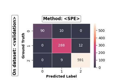
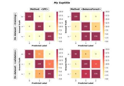
- confusion_matrix_heatmap(on_ensembles: list = None, on_datasets: list = None, false_pred_only: bool = False, sub_figsize: tuple = (4.0, 3.3), sup_title: bool = True, **heatmap_kwargs)[source]
Draw a confusion matrix heatmap.
- Parameters:
- on_ensembleslist of strings, default=None
The names of ensembles to include in the plot. It should be a subset of
self.ensembles_.keys(). ifNone, all ensembles fitted by the visualizer will be included.- on_datasetslist of strings, default=None
The names of evaluation datasets to include in the plot. It should be a subset of
self.eval_datasets_.keys(). ifNone, all evaluation datasets will be included.- false_pred_onlybool, default=False
Whether to plot only the false predictions in the confusion matrix. if
True, only the numbers of false predictions will be shown in the plot.- sub_figsize: (float, float), default=(4.0, 3.3)
The size of an subfigure (width, height in inches). The overall figure size will be automatically determined by (sub_figsize[0] * num_columns, sub_figsize[1] * num_rows).
- sup_title: bool or str, default=True
The super title of the figure.
if
True, automatically determines the super title.if
False, no super title will be displayed.if
string, super title will besup_title.
- **heatmap_kwargskey, value mappings
Other keyword arguments are passed down to
seaborn.heatmap().
- Returns:
- selfobject
- fit(ensembles: dict, granularity: int = None)[source]
Fit visualizer to the given ensemble models. Collect data for visualization with the given granularity.
- Parameters:
- ensemblesdict
The ensemble models and their names for visualization. The keys should be strings corresponding to ensemble names. The values should be fitted imbalance_ensemble.ensemble or sklearn.ensemble estimator objects.
Note: all training/evaluation datasets (if any) of all ensemble estimators should be sampled from the same task/distribution for comparable visualization.
- granularityint, default=None
The granularity of performance evaluation. For each (ensemble, eval_dataset) pair, the performance evaluation is conducted by starting with empty ensemble, and add
granularityfitted base estimators per round. IfNone, it will be set tomax_n_estimators/5, wheremax_n_estimatorsis the maximum number of base estimators among all models given inensembles.Warning
Setting a small
granularityvalue can be costly when the evaluation data is large or the model predictions/metric scores are hard to compute. If you find thatfit()is running slow, try using a largergranularity.
- Returns:
- selfobject
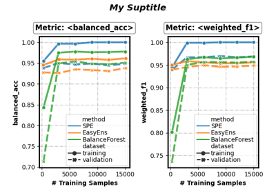
- performance_lineplot(on_ensembles: list = None, on_datasets: list = None, on_metrics: list = None, split_by: list = [], n_samples_as_x_axis: bool = False, sub_figsize: tuple = (4.0, 3.3), sup_title: bool = True, **lineplot_kwargs)[source]
Draw a performance line plot.
- Parameters:
- on_ensembleslist of strings, default=None
The names of ensembles to include in the plot. It should be a subset of
self.ensembles_.keys(). ifNone, all ensembles fitted by the visualizer will be included.- on_datasetslist of strings, default=None
The names of evaluation datasets to include in the plot. It should be a subset of
self.eval_datasets_.keys(). ifNone, all evaluation datasets will be included.- on_metricslist of strings, default=None
The names of evaluation metrics to include in the plot. It should be a subset of
self.eval_metrics_.keys(). ifNone, all evaluation metrics will be included.- split_bylist of {‘method’, ‘dataset’}, default=[]
How to group the results for visualization.
if contains
'method', the performance results of different ensemble methods will be displayed in independent sub-figures.if contains
'dataset', the performance results on different evaluation datasets will be displayed in independent sub-figures.
- n_samples_as_x_axisbool, default=False
Whether to use the number of training samples as the x-axis.
- sub_figsize: (float, float), default=(4.0, 3.3)
The size of an subfigure (width, height in inches). The overall figure size will be automatically determined by (sub_figsize[0] * num_columns, sub_figsize[1] * num_rows).
- sup_title: bool or str, default=True
The super title of the figure.
if
True, automatically determines the super title.if
False, no super title will be displayed.if
string, super title will besup_title.
- **lineplot_kwargskey, value mappings
Other keyword arguments are passed down to
seaborn.lineplot().
- Returns:
- selfobject